Key Performance Indicators
In order to assess current and future conditions in the Aa of Weerijs catchment, relevant indicators, named 'Key Performance Indicators (KPIs)' are chosen, in collaboration with the key stakeholders. These same indicators are used for assessing effectiveness of adaptation strategies consisting of Nature Based Solutions (NBSs). Primary KPIs are those associated with the hydrological condition in the catchment, in particular indicators for assessing water shortage / drought conditions.
The tabs below provide detailed explanations and examples of the KPIs selected for this pilot.
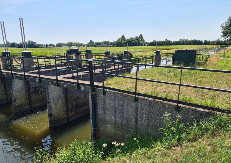
Control weir on Aa of Weerijs river - summer 2022
Description: This KPI provides information regarding the surface water available in the catchment, based on the mean daily flow available at a specific location. The Surface Water Availability (SWA) is determined by comparing the available flow at a specific location with some pre-defined threshold values and it is expressed in terms of number of days in which the discharge of interest is below (above) one of the thresholds. When the discharge drops below a certain level, the water managers exercise a ban on the extraction of surface water. According to the threshold that is crossed, the bans may be partial, i.e. targeting only specific activities, or total, i.e. prohibiting the abstraction for any kind of activities, with the exception of irrigation for capital-intensive crops.
This KPI is computed using the flows obtained from the simulations of a hydrological model under different scenarios: the base scenario, in which the model is forced with historical gauge-based observations in the period 2010-2019; climate change scenarios, in which the model is forced with the four climate change scenarios KNMI’23 for the decade 2050-2059; climate change with adaptation strategies (single-measure and combined), in which the hydrological model is forced with the HD (most extreme) climate change scenario for the decade 2050-2059 and, at the same time, some Nature-Based Solutions (NBS) are implemented in the model. The flows obtained in the base scenario are employed to compute the pre-defined thresholds used to evaluate the SWA, while the flows obtained in the climate change scenarios are used to compute the SWA in the decade 2050-2059, to assess the effects of climate change and of the adaptation strategies on the surface water.
The SWA is computed for some locations only, which correspond to the three locations in which there are currently installed monitoring gauges.
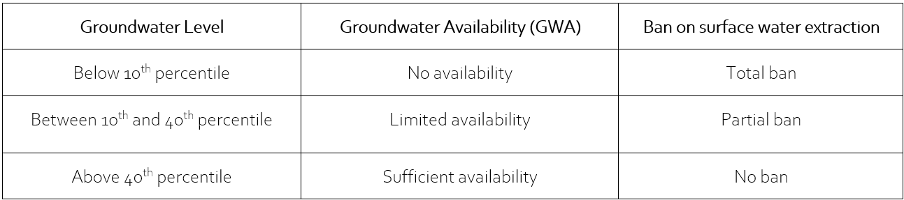
Definition: The Surface Water Availability (SWA) is defined as the number of days within a season in which the flow simulated at a specific location drops below a pre-defined threshold. Three different classes of surface water availability are defined: sufficient availability, limited availability and no availability. The SWA classes are identified for each location based on two thresholds: the 10th percentile and the 40th percentile, both referred to the flows obtained in the base scenario, at a specific location. The highest percentile rules the division between sufficient and limited availability, while the lowest rules the division between limited and no availability. The percentiles are calculated for each season of the year and the lowest among them are selected as thresholds for the computation of SWA. Moreover, each class of water availability corresponds to a ban condition: when simulated flow is in the sufficient availability class (i.e. above the 40th percentile), no ban is exercised; if simulated flow is in the limited availability condition (i.e. below the 40th and above the 10th percentile), a partial ban on extraction is exercised; in case the discharge is in the no availability class (i.e. below the 10th percentile), a total ban is applied on water extraction activities. The different classes, bans and thresholds are summarized in the table below:

Computational procedure: This KPI is computed through the following steps:
- Compute the thresholds that define the three water availability classes:
- Gather the flows simulated at a specific location in the base scenario over a specific season, for at least 10 years;
- Compute the 10th and 40th percentile of the data collected in point a;
- Repeat steps 1a-1b for all the seasons;
- Select the lowest thresholds among those computed for the four seasons and use them to define the water availability classes.
- Compute the KPI:
- Define the forcing scenario and the season for which to compute the KPI and collect the simulated flow for that period;
- Compare the data collected at step 2a with the specific thresholds defined in step 1d;
- Count the number of occurrences (days) in which the discharge collected in 2a belongs to a specific water availability class;
- Repeat steps 2a-2c for all the seasons of interest.
- Time series of the mean daily discharge simulated in the base scenario at a specific location of at least 10 years length for determining the thresholds. Such a time series length is needed in order to include a variety of samples corresponding to wet, dry and normal hydrological years.
- Time series of simulated mean daily discharge at a specific location for the scenario of interest, for at least a season length.
Intended use of information: The information can be used to examine the impact of climate change and different adaptation strategies on surface water availability or streamflow in comparison with historical base conditions.
Spatial extent: The SWA is assessed at three locations: at the catchment outlet, middle and close to the Belgian border.
Output format: The KPI is provided both in the form of a time series plot and of a bar chart, respectively showing discharge timeseries and the number of days within a season in which water is sufficiently available, available with limitations or not available for extraction, as shown in the example figure.
In the example, the first box from the top shows the time series of flow simulated at the catchment outlet in the decade 2010-2019. The background coloured bands show the ranges of values in which the flow belongs to the classes of sufficient availability (green area), limited availability (orange area), and no availability (red area). The second box identifies all the days over the same period in which the flow resulted to be in the limited availability (orange lines) and in the no availability (red lines) classes. The third box from the top shows the SWA for each season of the year, accumulated over the decade 2010-2019. For instance, the summer bars indicate the total number of days over the summer periods 2010-2019 in which water was sufficiently, limitedly or not available for extraction. Finally, the bottom box presents the daily flow time series zoomed over summer 2018, which resulted to be the driest season over the base scenario.
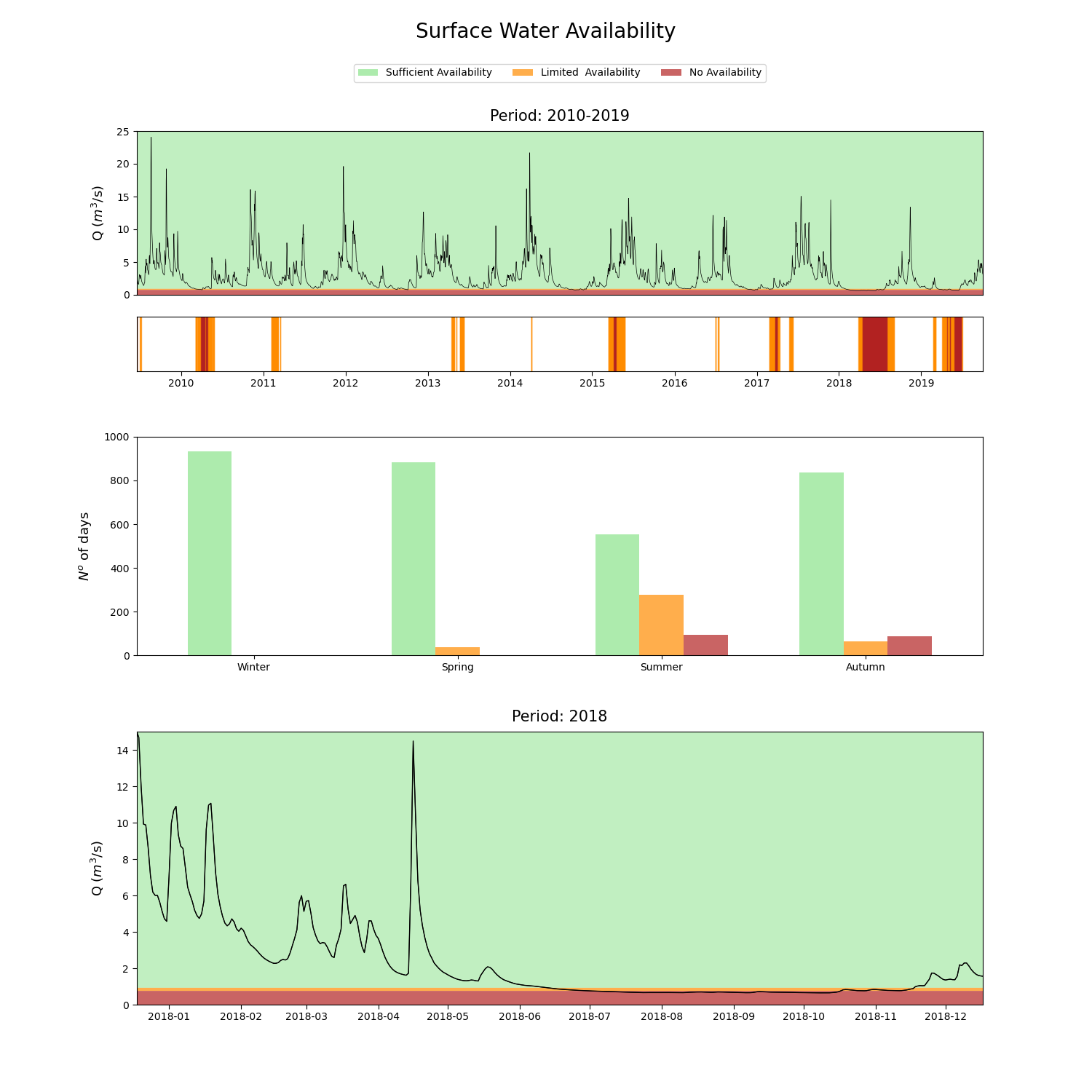
Example SWA results for the base case scenario
Description: This KPI provides information about the groundwater availability in the catchment, based on groundwater levels. The Groundwater Availability (GWA) is determined by comparing the groundwater level at a specific grid cell with some pre-defined thresholds based on long term groundwater variations at that point and it is expressed in terms of number of days in which the groundwater level is below (above) one of the thresholds. When the groundwater level drops below a certain threshold, the water managers exercise a ban on the extraction of water. According to the threshold that is crossed, the bans may be partial, i.e. targeting only specific activities, or total, i.e. prohibiting the abstraction for any kind of activities, with the exception of irrigation for capital-intensive crops.
This KPI is computed using the groundwater levels obtained from the simulations of a hydrological model under different scenarios: the base scenario, in which the model is forced with historical gauge-based observations in the period 2010-2019; climate change scenarios, in which the model is forced with the four climate change scenarios KNMI’23 for the decade 2050-2059; climate change with adaptation strategies (single-measure and combined), in which the hydrological model is forced with the HD (most extreme) climate change scenario for the decade 2050-2059 and, at the same time, some Nature-Based Solutions (NBS) are implemented in the model. The groundwater levels obtained in the base scenario are employed to compute the pre-defined thresholds used to evaluate the GWA, while the levels obtained in the climate change scenarios are used to compute the GWA in the decade 2050-2059, to assess the effects of climate change and of the adaptation strategies on the groundwater resources. The GWA is computed for some locations only, which corresponds to the locations in which there are currently monitoring wells.
Definition: The Groundwater Availability (GWA) is defined as the number of days within a season in which the groundwater level simulated at a specific well in the catchment drops below a specific threshold. Three different classes of GWA are defined: sufficient availability, limited availability and no availability. The classes are identified based on two thresholds: the 10th percentile and the 40th percentile, both referred to the groundwater levels obtained in the base scenario, at a specific location. The highest percentile rules the division between sufficient and limited availability, while the lowest rules the division between limited and no availability. The percentiles are calculated for each season of the year and the lowest among them are selected as threshold for the computation of GWA. Moreover, each class of water availability corresponds to a ban condition: when simulated level is in the optimal availability class (i.e. above the 40th percentile), no ban is exercised; if simulated level is in the limited availability condition (i.e. below the 40th and above the 10th percentile), a partial ban on extraction is exercised; in case the groundwater level is in the no availability class (i.e. below the 10th percentile), a total ban is applied on groundwater extraction activities. The different classes, bans and thresholds are summarized in the table below:
Computational procedure:This KPI hi is computed through the following steps:
- Compute the thresholds that define the three groundwater availability classes:
- Gather the groundwater levels simulated at a specific location in the base scenario over a specific season, for at least 10 years;
- Compute the 10th and 40th percentile of the data collected in point a;
- Repeat steps 1a-1b for all the seasons;
- Select the lowest thresholds among those computed for the four seasons and use them to define the groundwater availability classes.
- Compute the KPI:
- Define the forcing scenario and the season for which to compute the KPI and collect the groundwater levels simulated for that period;
- Compare the data collected at step 2a with the specific thresholds defined in step 1d;
- Count the number of occurrences (days) in which the water level collected in 2a belongs to a specific groundwater availability class;
- Repeat steps 2a-2c for all the seasons of interest.
- Time series of simulated mean daily water level at the location of interest over the base scenario, of at least 10 years length for determining the thresholds. Such a time series length is needed in order to include a variety of samples corresponding to wet, dry and normal hydrological years.
- Time series of observed mean daily groundwater levels at that location for the period of interest.
Intended use of information: The information can be used to examine the impact of climate change and different adaptation strategies on groundwater availability in comparison with base conditions.
Spatial extent: This KPI is provided at 13 specific locations, which corresponds to the existing monitoring wells.
Output format: The KPI is provided in the form a time series plot and a bar chart, showing water level timeseries and the number of days within a season in which water is sufficiently available, available with limitations or not available, as shown in the example.
In the example, the first box from the top shows the time series of groundwater levels simulated at the monitoring well B50C0079 (located in modelling cell 27_32) in the decade 2010-2019. The background coloured bands show the ranges of values in which the groundwater level belongs to the classes of sufficient availability (green area), limited availability (orange area), and no availability (red area). The second box identifies all the days over the same period in which the groundwater levels resulted to be in the limited availability (orange lines) and in the no availability (red lines) classes. The third box from the top shows the GWA for each season of the year, accumulated over the decade 2010-2019. For instance, the summer bars indicate the total number of days over the summer periods 2010-2019 in which groundwater was sufficiently, limitedly or not available for extraction. Finally, the bottom box presents the daily groundwater level time series zoomed over summer 2018, which resulted to be the driest season over the base scenario.
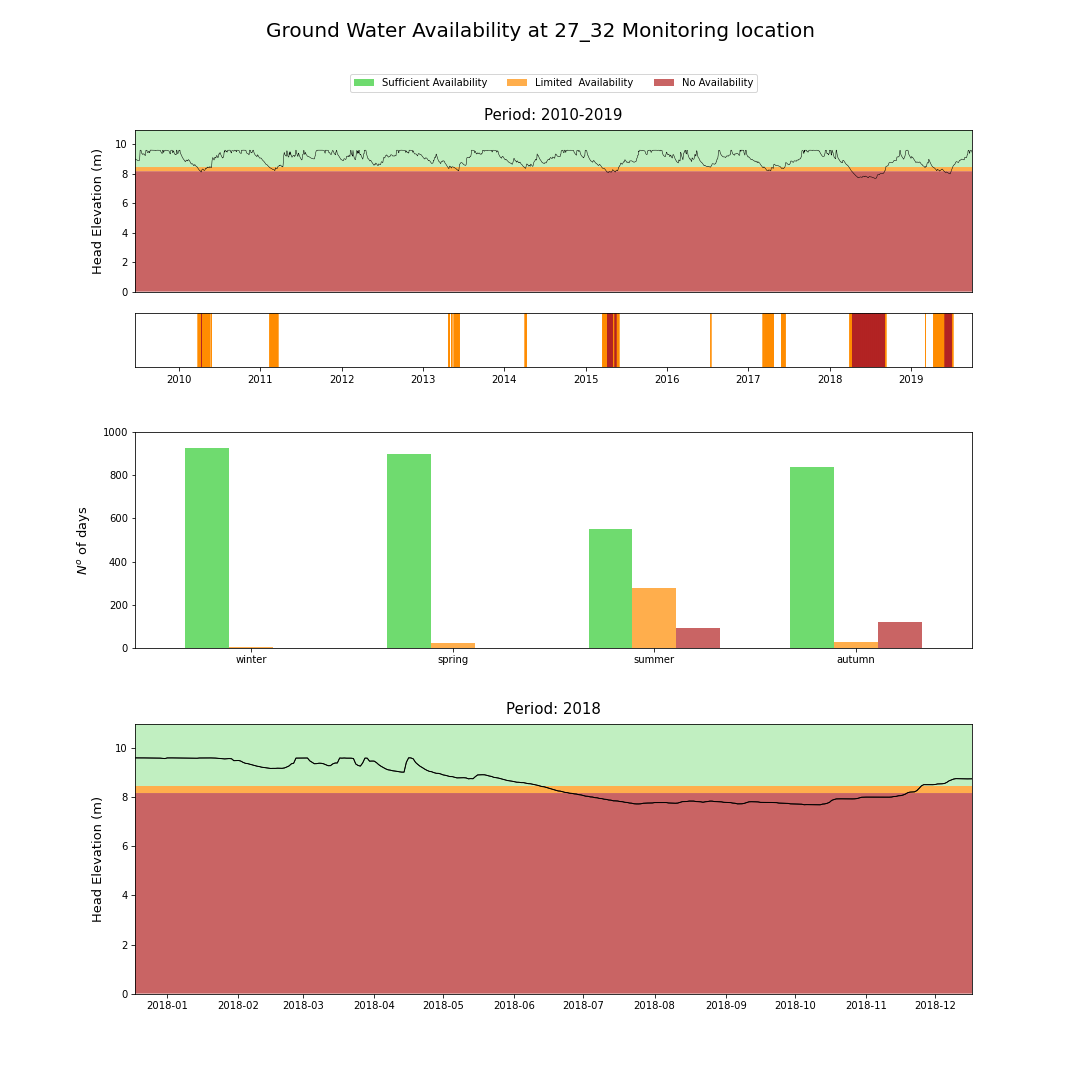
Example GWA results for the base case scenario, for one of the monitoring wells.
Description: The Soil Moisture Index (SMI) assesses the moisture content in the soil. It provides valuable information about water availability for plants and ecosystems.
This KPI is computed using the soil moisture values obtained from the simulations with the hydrological model under different scenarios: the base scenario, in which the model is forced with historical observations in the period 2010-2019; climate change scenarios, in which the model is forced with the four climate change scenarios KNMI’23 for the decade 2050-2059; climate change with adaptation strategies (single-measure and combined), in which the hydrological model is forced with the HD (most extreme) climate change scenario for the decade 2050-2059 and, at the same time, some Nature-Based Solutions (NBS) are implemented in the model. The SMI is computed both for every grid cell of the hydrological model domain and as average over the catchment.
Definition: The Soil Moisture Index is defined as shown in Equation 2 below, adopted from Sahbeni, et al. (2023):
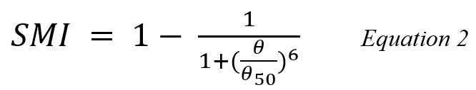
where θ is the mean soil moisture content and θ_50 is the average between the wilting point and field capacity. A SMI value of 0 indicates dry conditions, whereas a score of 1 indicates wet conditions in the unsaturated zone (Saha, et al., 2018). This same definition has also been adopted by the European Centre for Medium-Range Weather Forecast (ECMWF) for calculating soil moisture anomaly using the hydrological model LISFLOOD at the European scale.
Computational procedure: The Soil Moisture Index is computed using Equation 2, as described in Sahbeni et al. (2023), in every grid cell of the catchment. The mean soil moisture θ is computed as the average between the water content at 10 cm and 20 cm depth, while the values of θ_50 are computed as the average of the field capacity and the wilting point, according to the soil type present in every grid cell. The soil properties for each soil type are obtained using the Rosetta model of USDA for hydraulic parameters of soils. The SMI is calculated both for each of the summer months (June, July and August) and as an average over the whole summer season. It is available both in every grid cell and as an average over the catchment, in the latter case using the catchment average water content in the unsaturated zone in the equation presented above.
Required data:
- Time series of water content at the layers with 10 cm and 20 cm depth, for the period of interest;
- Field capacity and wilting point of each soil type, in order to calculate SMI in each of the grid cell;
- Soil properties for each soil type.
Intended use of information: The SMI data can contribute to water resource planning and management strategies. Indeed, by analysing the SMI values across different regions or catchments, water managers can assess the overall soil moisture conditions and make informed decisions regarding water allocation, drought management, and water conservation measures.
Spatial extent: The SMI is available both fully distributed in every grid cell and as a spatial average over the catchment.
Output format: This KPI is provided both in the form of a timeseries graph showing the average values at catchment level, and as a map showing the soil moisture index at each catchment grid cell, as shown in the example figures. In the former case, the time series depict the monthly average values over the scenario of interest, while in the latter case the maps present the average values over the summer months (June, July, August) and the entire summer season over the scenario of interest.
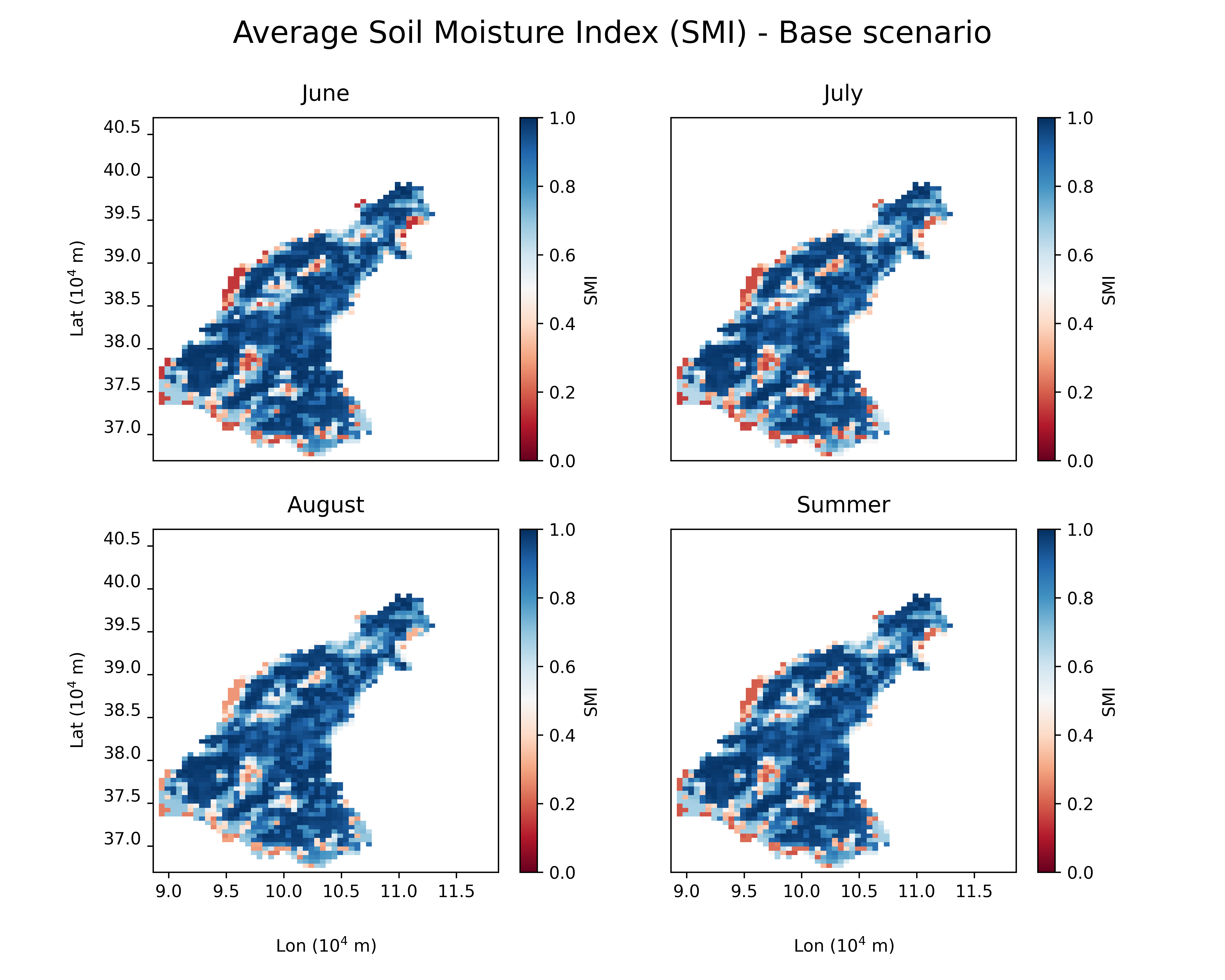
Average SMI for June, July, August and the whole summer - Base scenario
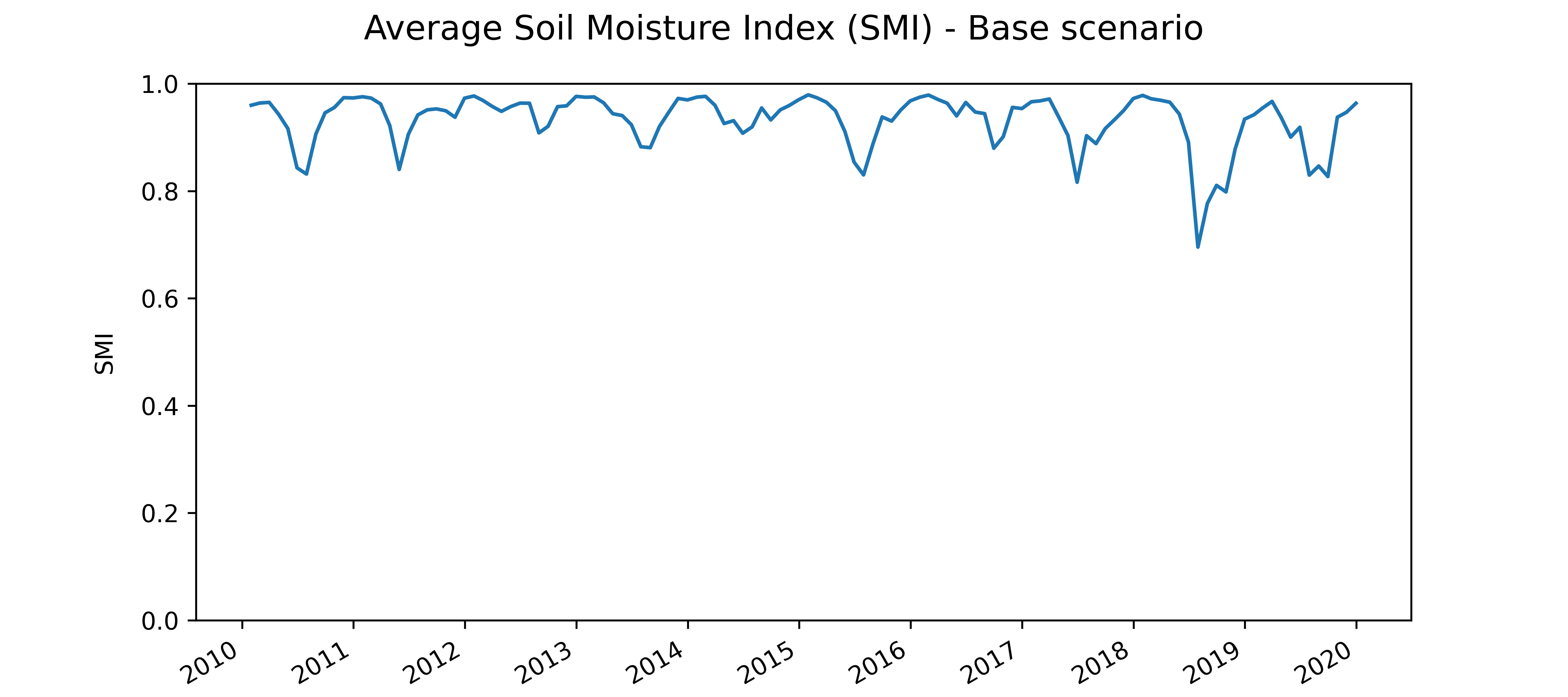
Time series of SMI spatially averaged over the whole catchment - Base scenario
Description: The groundwater dynamics can be assessed by looking at the average highest groundwater level (GHG), average spring groundwater level (GVG), and average lowest groundwater level (GLG). The study of these levels provides insights into the overall variability and range of groundwater levels in a catchment, allowing for a comprehensive understanding of groundwater dynamics and their potential impacts on water resources.
This KPI is computed using the groundwater levels obtained from the simulations with the hydrological model under different scenarios: the base scenario, in which the model is forced with historical observations in the period 2010-2019; climate change scenarios, in which the model is forced with the four climate change scenarios KNMI’23 for the decade 2050-2059; climate change with adaptation strategies (single-measure and combined), in which the hydrological model is forced with the climate HD (most extreme) change scenario for the decade 2050-2059 and, at the same time, some Nature-Based Solutions (NBS) are implemented in the model.
Definition: The groundwater dynamics parameters (GXG) is the set of the average highest groundwater level (GHG), average spring groundwater level (GVG), and average lowest groundwater level (GLG).
Computational procedure:
The average highest (lowest) groundwater level is computed as follows:
- Collect the time series of groundwater levels simulated over a period of 10 years;
- For each hydrological year (1st April – 31st March), select the groundwater levels simulated twice a month (14th and 28th of each month);
- For each hydrological year, select the three highest (lowest) groundwater levels among those collected in step 2 and average them. At the end of this step, 10 average values are obtained;
- Average the values obtained at step 3 to obtain the average highest (lowest) groundwater level GHG (GVG).
- Collect the time series of groundwater levels simulated over a period of 10 years;
- For each hydrological year (1st April – 31st March), select the groundwater levels simulated on 14th March, 28th March and 14th April, and average them. At the end of this step, 10 average values are obtained;
- Average the values obtained at step 2 to obtain the average spring groundwater level GVG.
Required data: Time series of head elevation in saturated zone obtained from the hydrological model runs, of at least 10 years length.
Intended use of information: The GXG can be used as input for the nature and agriculture impact models, providing information whether the groundwater status is optimal, too wet or too dry for the local vegetation. Moreover, the GXG values can be compared over different forcing scenarios, to identify hotspots in the catchment, and to examine how climate change and adaptation strategies are influencing the groundwater.
Spatial extent: This KPI is available in every grid cell of the catchment.
Output format: This KPI is provided in a form of a map, showing the GXG values in every grid cell of the domain. An example is provided in the figure below, where the left panel shows the highest groundwater levels (GHG), the central panel shows the lowest groundwater levels (GLG) and the right panel shows the spring groundwater levels (GVG).
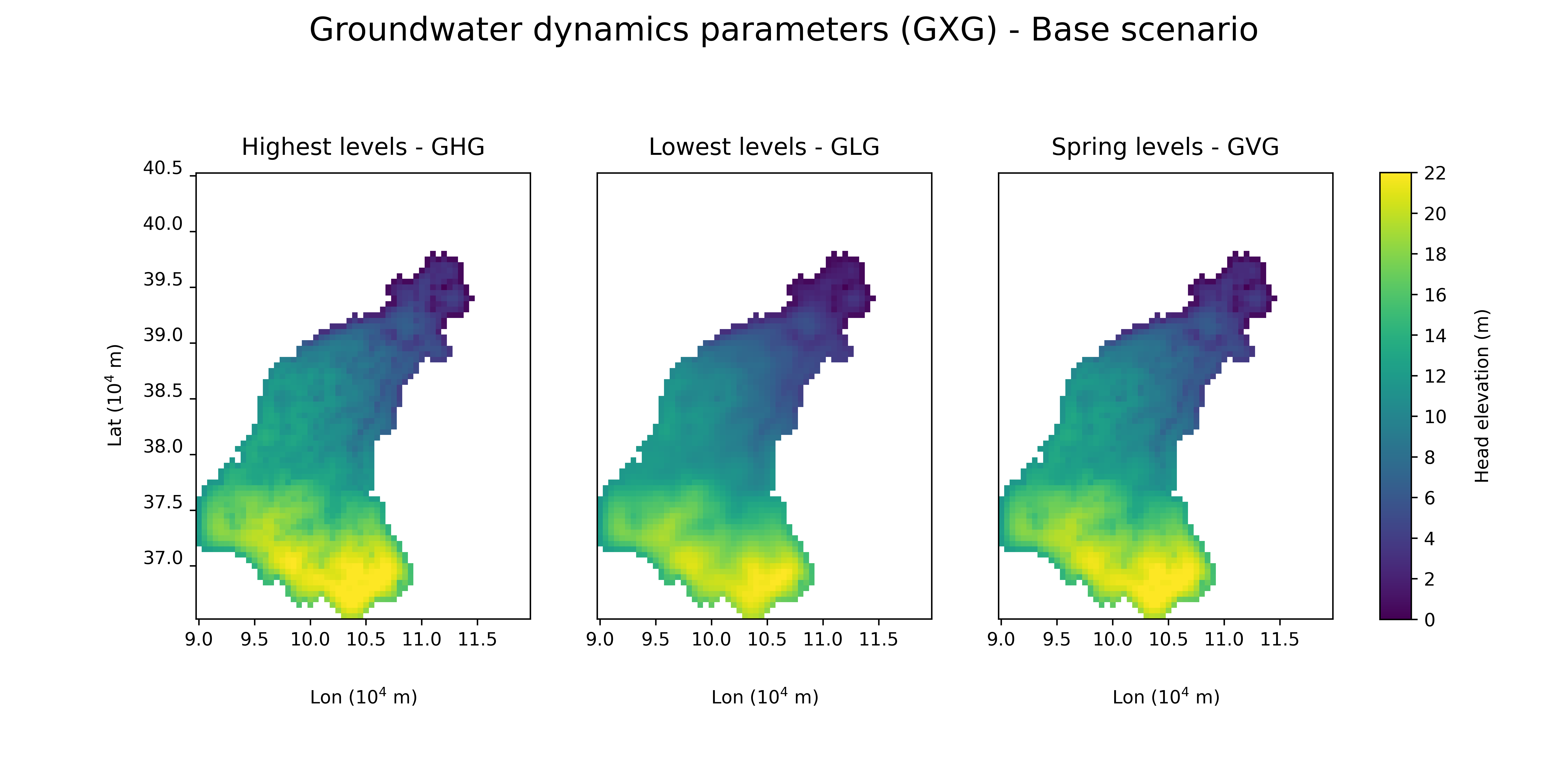
Example GXG results for the base scenario
Description: The hydrological model provides several output time series in every grid cell of the catchment, such as groundwater levels, soil moisture, actual evapotranspiration, and discharge or surface water levels in the river network. Some of these Localized Model Outputs (LMO) are available for direct inspection at specific locations.
The LMO are obtained from the simulations of the hydrological model under different scenarios: the base scenario, in which the model is forced with historical observations in the period 2010-2019; climate change scenarios, in which the model is forced with the four climate change scenarios KNMI’23 for the decade 2050-2059; climate change with adaptation strategies (combined), in which the hydrological model is forced with the HD (most extreme) climate change scenario for the decade 2050-2059 and, at the same time, some Nature-Based Solutions (NBS) are implemented in the model.
Definition: The LMO provided here are avreage weekly time series of groundwater levels and river discharges, in different forcing scenarios, as outputs of the hydrological model runs.
Computational procedure: The variables included in this KPI are the direct model output at a spatially distributed scale for the whole simulation domain. Information on the computation procedure and the hydrological processes involved can be found in the MIKE SHE documentation.
Required data: Gridded model output for the variables of interest.
Intended use of information: The local time series can be analysed to understand the hydrological behaviour of the catchment. Moreover, time series can be compared under different forcing scenarios, to assess the impacts of a change in the climate forcing and of adaptation strategies, helping to identify the most vulnerable points in the catchment.
Spatial extent: This KPI is available in selected locationss within the catchment, corresponding to existing monitoring locations of groundwater levels and river discharges.
Output format: This KPI is provided in the form of a timeseries graph for each selected location. The two example figures show the time series of river discharge at the catchment outlet and groundwater levels for the location of the monitoring well B50C0079 (located in modelling cell 27_32), for the base and HD CC scenarios.
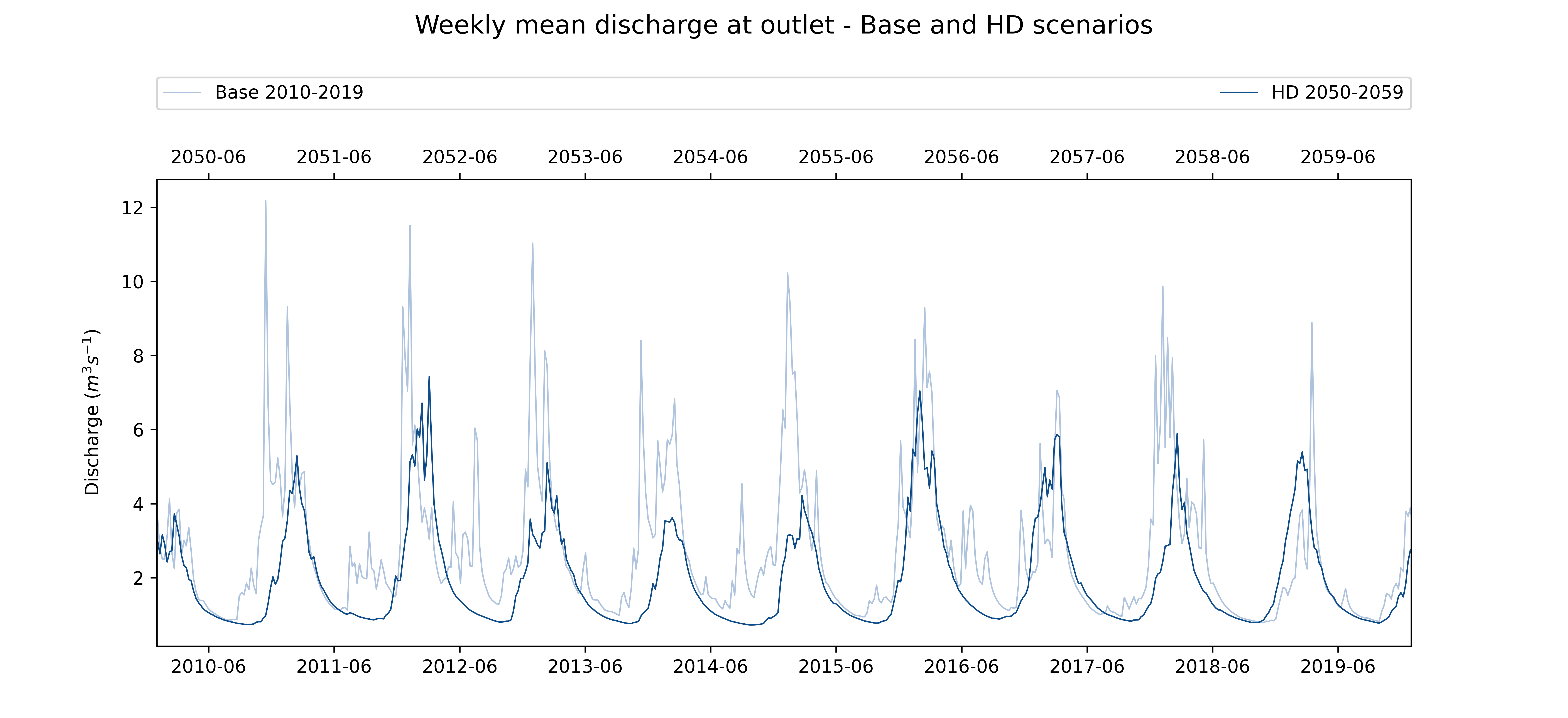
Example river discharge results for one location - base and HD scenarios
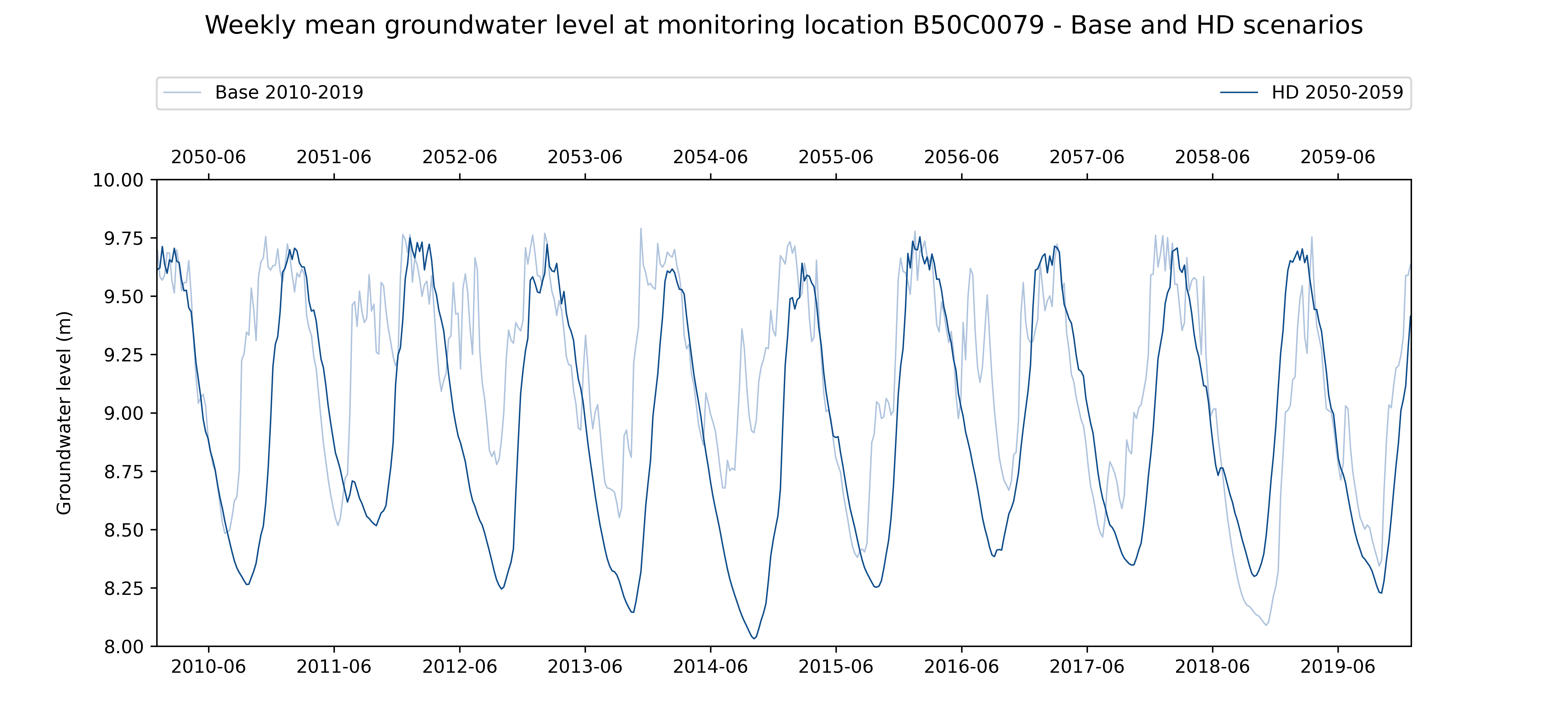
Example Groundwater level results for one location - base and HD scenarios
Description: The Soil Organic Carbon Difference (SOCD) is a key performance indicator used to measure the effectiveness of nature-based solutions or adaptation and mitigation strategies aimed at restoring and enhancing soil carbon levels in a degraded area. Soil carbon sequestration is a crucial process that involves the capture and storage of atmospheric carbon dioxide (CO2) in the soil through natural or human-induced means. The SOCD provides valuable insights into the success of these efforts to mitigate climate change and enhance ecosystem health by increasing soil organic carbon content.
Definition: SOCD is the quantification of the increase or decrease in Soil Organic Carbon (SOC) content (%) per grid cell in an alternative scenario (e.g. NBS) as compared to the value of SOC (%) in the same grid cell for its existing situation (ES). It is expressed in terms of carbon percentage for a specific soil texture when its original carbon stock (kg/ha), is transformed to percentage using the bulk density (BD) for the soil texture in that grid cell.
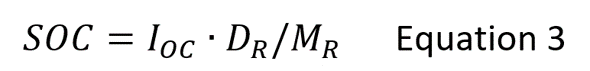
where IOC = input of organic carbon (kg/ha); DR = decomposition rate (%) and MR = mineralization rate (%); SOC (kg/ha).

where SOCNBS is the modelled SOC (%) for an NBS scenario and SOCES is the modelled SOC (%) for the existing situation of the catchment.
Computational procedure: The SOCD is computed as follows:
- Baseline Assessment: Run a carbon model coupled with a hydrological model using at least 2 iterations between the models and using the comprehensive survey data for the analysis of the input of the soil organic carbon content of the existing situation in the area before implementing any nature-based solutions or adaptation and mitigation strategies. This baseline data will serve as a reference point for calculating the difference.
- NBS Assessment: Run a carbon model coupled with a hydrological model using at least 2 iterations between the models for the NbS.
- Calculate Net Change: Compute the net change in soil carbon per grid size per soil texture type.
- Express as SOCD: Convert the stock change (kg/ha) to soil carbon content (%)by using the BD calculation from Wosten (1999) for the specific soil texture in that grid.
Required data:
- Average soil moisture map of the catchment for the whole MIKE duration period (10 years) up to 30cm depth
- Carbon Input based on existing soil survey data
- Average Soil Temperature
- Soil properties for each soil type
Spatial extent: The SOCD is available fully distributed in every grid cell
Output format: This KPI is provided in a form of a map, showing the SOCD values in every grid cell of the domain.
Note: This KPI has been calculated for three single-measure adaptation strategies: tree planting, heathland restoration and wetland restoration. One additional case with extreme reforestation in the whole Aa of Weerijs catchment has also been tested, for which the example calculations are presented in the figure below.
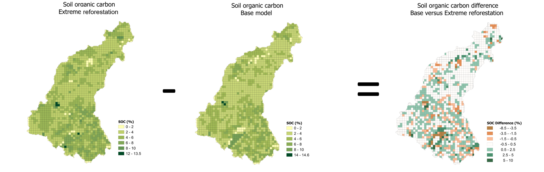
Example SOCD calculations for extreme reforestation strategy versus the base model (current conditions)